Handwritten digit recognition – Part1

OBS: There is a version in portuguese.

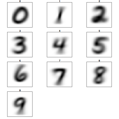
Handwritten digit recognition task was one of first great successes of machine learning methods. Nowadays, the task can be carried out by multiple specialized libraries with very high accuracy (> 97% of correct answers), such that many times, despite of indirectly we use these features in tablets and smartphones, in general we do not know exactly how the method works.

Thinking about it, as I worked with this problem before, I will demonstrate in this post how the process works, the techniques used and how to implement it with R language. To begin, we will work with the problem of recognizing digits 0,1,2 , 3,4,5,6,7,8, or 9, i.e. a classification problem with 10 categories.

I’ll try to work here implementing all the modeling only with R base functions and a few extra packages with the required functions and algorithms; in the next post, I can try to use other packages to automate the various modeling tasks.

1. READING DATA

The dataset is images of the type PGM, with 64 x 64 pixels per image, where each pixel has a value of 1 or 0, indicating whether the pixel is black or white. Each image has a name as X_ yyy.BMP.in.pgm, where X represents the digit drawn in the image. The data are divided into a training set and a test set and can be downloaded from the following links: teste  e treino (test and trainning; save with any name you want).

Thus, the first part of the problem is reading the data. For this I will use pixmap package with which you can read and manipulate PGM images. Next, the process of reading the images and creation of an array with the labels, that is, the number that is written in the image.

## Load pixmap
library(pixmap)

## Def working directory
path_treino <- '/sua/pasta/treino/'

## Set wd
setwd(path_treino)

## Read files
files <- dir()

## Getting classes from file names
classes <- as.factor(substring(files,first=1,last=1))

## Trainning data.frame
treino <- as.data.frame(matrix(rep(0,length(files)*64*64), nrow=length(files)))

## Reading trainning dataset
for (i in 1:length(files)) {

  ## Reading images
  x <- read.pnm(files[i])

  ## Slot 'grey' with pixels; the matrix is vectorized
  treino[i,] <- as.vector(x@grey, mode='integer')
}

## Same for test set
path_teste <- '/sua/pasta/teste/'

## Same for teste set
setwd(path_teste)

## Same for test set
files <- dir()

## Classes
predic <- as.factor(substring(files,first=1,last=1))

## Data.frame for test set
teste <- as.data.frame(matrix(rep(0,length(files)*64*64), nrow=length(files)))

## Reading test set
for (i in 1:length(files)) {
  x <- read.pnm(files[i])
  teste[i,] <- as.vector(x@grey, mode='integer')
}

Note that the pixel array is stored @grey slot, and after reading, it is transformed into a vector, such that the final data.frame has 64×64 columns and 1949 rows (images total). The test set is only 50 images, so the data.frame will stay with 64×64 columns and only 50 lines. In summary, each column is a pixel and each line is an image.

 2. MODELLING WITH k-nn

At this step we will create models with the k-nn algorithm (nearest neighbors) without any data preprocessing. The algorithm works by assigning classes to images, using the known values of the closest neighbors. So, lets say k = 3, the algorithm looks for the three nearest images, checks the majority class of these images and assign this class to the image without label. It is important to choose an odd k to prevent draw, for example, two neighbors of a class and another two from other, in the case of k = 4.

## Package with knn
library(class)

## knn model with k=3
predito <- knn(train=treino, test=teste, cl=classes, k=3, prob=T)

## Results
result <- data.frame(cbind(predic, predito, acerto = predic==predito))

## Accuracy
sum(result$acerto)/nrow(result)

[1] 0.56

And with k = 3 we got a success rate of only 56%, far short of what can be achieved. So let’s run the algorithm with different k values and see if we can get a result a little better.

## Data.frame all results
resultado <- data.frame(k = rep(0,101), taxa=rep(0.00,101))

for (i in seq(from=1, to=101, by=2)) {
  
  ## Print k values 
  print(i)
  
  ## Predicted images
  predito <- knn(train=treino, test=teste, cl=classes, k=i, prob=T)
  
  ## Save data.frame
  result <- data.frame(cbind(predic, predito, acerto = predic==predito))
  
  ## Accuracy; store at the data.frame
  resultado[i,] <- c(i,sum(result$acerto)/nrow(result))
}

## Get rid of blank lines
resultado <- subset(resultado, subset=resultado$taxa!=0)

## Ploting results for all k's
plot(resultado$taxa~resultado$k, main='Taxa de Acerto para o k-nn', xlab='Valores de K', ylab='Taxa de acerto')

We got something like 78% with k = 1, but it is still a very poor result close to what can be achieved. It is also worth noting that increasing K does not help much in the end, but it is important to be aware that a very small k can lead to overfitting.

CONCLUSION

 Apparently handwriting recognition works well using a simple algorithm, without any treatment. HOWEVER, we can do better. In Part 2 we will automate some tasks with caret package and we will also explore other better algorithms such as SVM and RandomForest.